SQL For Data Science: A Comprehensive Beginners Guide

In this blog, I am going to talk about the importance of SQL for data science, some statistics, and key concepts that you need to be aware of as a beginner in pursuit of a data scientist career path.

I have also covered some of the key SQL practices that have to be followed when working with data.

You will also learn the fundamentals of SQL and working with data so that one can begin analyzing it for data science purposes

SQL – Data Science Statistics

Data Science has emerged as the most popular field of the 21st century. It is because there is a pressing need to analyze and construct insights from the data. Industries transform raw data into furnished data products.

To do so, it requires several essential tools to churn the raw data. Collectively with Python and R, SQL is now considered to be one of the most demanded skills in Data Science.

As per KDnuggets, SQL is the third skill in demand for data scientist jobs.

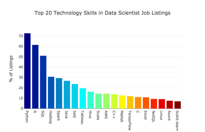
SQL isn’t going anywhere. Yes, it’s true. SQL is more popular amongst data scientists and data engineers than R or Python. The truth that SQL is a language of choice is incredibly significant.

In the chart below, from recent StackOverflow’s 2020 developer survey, one can see that SQL eclipses both Python and R in popularity.

What’s SQL?

Structured Query Language (SQL) is a database language used to create, retrieve & manipulate the data from a Relational Database Management System (RDBMS) such as MySQL, Oracle, SQL Server, Postgre, etc. that stores the data in relational database tables.

The relational database table consists of columns and rows, where columns describe the stored data’s properties, and rows describe the real data entries.

As the name suggests, SQL comes in to picture when we have structured data, e.g., in the form of tables.

On the other hand, the databases that are not well structured or not relational, and therefore do not use SQL are known as NoSQL databases. Examples of such databases are MongoDB, DynamoDB, Cassandra, etc.

Some interesting facts about SQL that should Know

• One of the interesting facts about SQL is that it’s made up of descriptive words. In other words, most of the commands used in SQL are reasonably easy to understand as compared to many other computer languages. It makes SQL, as a language, really simple to read and learn. For example, one wants to select a column NAME from the STUDENT table. Then he/she can write the SQL command as

SELECT NAME FROM STUDENT;

• SQL statement keywords are case sensitive. It means that

SELECT ROLL_NO, NAME FROM STUDENT;

is not similar to,

Select ROLL_NO, NAME From STUDENT;

• There is an ISO standard for SQL; most of the implementations lightly differ in syntax. So one may encounter queries that work in SQL Server but do not work in MySQL.
• SQL is a non-procedural language that means we can’t write a complete application using SQL, but what you can do is interact and communicate with data. It makes it relatively simple, but also a clear language.

Why SQL for Data Science?

1. According to research, more than 2.5 quintillion bytes of data are produced every day. Hence for storing such vast amounts of data, it is strictly needed to make use of databases.
2. Industries are now giving more importance to the value of data. Data can be used in various ways to analyze more significant business problems, solve business problems, make predictions, and understand customer needs.
3. While performing manipulations on data, SQL can be accessed directly, and this is one of the main advantages of using SQL because this can expedite the workflow executions.

Before deep dive into SQL, prior knowledge in Relational Model, Some important terminologies related to the relational model, and keys in the relational model are essential for the beginners.

Using SQL for Data Science

So now, the question is, how do you bring SQL together for use in data science?

Every data science project starts with the aim of finding a solution to a problem.

These are a few approaches and standard practices followed when beginning with a new data science problem that requires SQL.

As a beginner, it’s essential to know how to work through a problem from beginning to end.

Here we are going to discuss the key practices that have to be followed before starting to write SQL queries for any data science-related projects.

1. Understanding Data
2. Understanding the Business Use Case
3. Data Profiling
4. Troubleshooting
5. Data Formating
6. Review Process

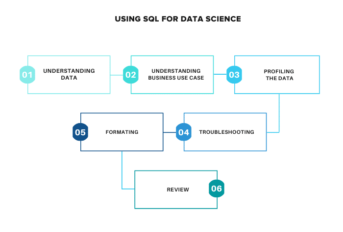
Let’s understand each stage in detail.

Data Understanding

So the very first step is data understanding, and it is the most crucial step. It is why you need to spend enough time modeling diagrams, discussing the associations in the data, because knowing the data is key to writing successful queries.

It’ll be very beneficial to kill the time to know the data as much as possible before interpreting it. It’s essential to know the associations and dependencies among the data.

That drives us to our second step, which is business understanding.

Business Understanding

As we start to get familiar with the data, what happens, is that we move into questions regarding the business problem that we are striving to solve. 

Usually, one will be moving back and forth to study at the data and move back to a subject matter specialist who knows the core business problem and strives to resolve it. 

This is crucial in being capable of wrapping your head around the problem.

One of the things to be aware of is the unspoken need. There may be a business problem; for example, one wants to predict whether or not a customer is expected to buy the product. 

That looks pretty straightforward and easy. But as one falls into the data more, he/she may start to get questions like which customers? Which products? Some of the unspoken points are specific logical exclusions.

If you can get this and understand a problem, query writing will just become more comfortable. If you genuinely know the data and understand the problem, then writing the queries is like filling in the blanks.

Profiling Data

When we are trying to understand the data, we will start profiling the data. This is where we perform descriptive statistics.

It’s also a significant opportunity to classify any data quality issues before diving into the analysis. It’s a good approach to perform this profiling step before finalizing any of the data that we are extracting.

To catch a problem, we require a plan of what are the exact data components we need.

We require to understand the data we are working on going after and get some of the data from the profiling we have done.

If we are regularly obtaining the data, then it will begin with the select statement. So we have to use select and from.

Start with Select

Remember, you’re always going to start with the SELECT statement. It means that’s the great thing about SQL, it’s consistent in that way.

It is recommended to start simple, particularly if you’re new to the data. Begin with just one table, add more data, add in another table, check the result, and then go back from there.

If you’re using subqueries, remember to always start with the innermost query and then work out and build. That drives to the next point, which is a test along the way.

Test & Troubleshoot

Don’t wait to test the query until we have combined various sources. And we have all our calculations done and completed. Think of these as little building blocks.

If we write an estimation of something’s average selling price, look at how many values we are getting back for that calculation from the table and make sure that appears right.

Then combine the result with different tables and then examine that. If we understand the data, we could jump in a little bit faster. But make sure that our order of manipulation is accurate.

It is important because it’s simple to get results back, but taking the correct results back that we require is a little bit harder.

Troubleshooting is necessary always to start short and simple, and slowly start to reconstruct the query to see where things went wrong. It’s essential to start with the basic things first.

Gradually start to develop a backup to understand where things have gone wrong.

Format & Comment

Be sure that when we are writing the query, the next thing to look at is to make sure we are formatting it accurately and commenting correctly.
The clean code says a lot about the coder.

Ensure that it’s easy to read the query, use recommended indentation, comment strategically where we need to do so, etc.

We never know when we will require to revisit the query, or we are going to require to deliver it to someone else, and they need to update it from there.

Just keep the code clean. Format the comments where necessary and strategically.

Review

Now make sure that we have reviewed what we have done till now. A lot of times, what happens is we write the query, we will be using it for our model, and we will be looking at various stats and stuff like that.

Then we need to go back and change that query. Always make sure to review the query to see if anything has changed. Has the data changed? Are business rules different? Do we require updating the date indicators?

And be cautious when you’re going back and using old queries.
These approaches take us over a problem from start to end, and it all begins with the data and problem understanding.

Make sure to spend the time there. Make sure to spend the time thinking about what we are doing before we start writing the queries.

And it’s going to save our time in the long run, then go through and understand the data by profiling it. Make sure to test enough and keep the code clean with proper commentation.

DBA vs Data Scientist

Many use SQL in their jobs. This includes everything from backend developers, QA engineers, system engineers, obviously data scientists, and even data analysts. But the one we want to know about more is the DBA (Database Administrators), and how he/she compares to data scientists.

The DBA is responsible for managing the whole database and supervising it. However, the data scientist is typically a user of that database. The DBA will be responsible for granting permissions to people and deciding who has access to what data. They’re often responsible for managing the tables and creating them. 

DBAs and data scientists are related to each other in such a way that they both use SQL to interpret the data, to query it, and retrieve it. They both write quite complex queries, but the main difference is that the data scientist is the end-user. However, the DBA is the one who manages it, directs it, and maintains the database as a whole.

Relational Model in DBMS

Now, let’s start with the practical basics to understand the underlying concepts of a relations model.

The relational model illustrates how data is stored in relational databases.  The data is stored in the form of relations or tables in a relational database. Suppose a table STUDENT having attributes or characteristics ROLL_NO, NAME, PHONE, and AGE shown in the following table.

STUDENT TABLE

ROLL_NO	NAME	PHONE	AGE
1	Asish	9438351764	25
2	Raj		30
3	Sidhu	8908987865	40
4	Emraan	7658908765	25

Important Terminologies

1. Relation Schema: A relation schema depicts the name of the relation with its attributes. e.g.; STUDENT (ROLL_NO, NAME, PHONE, and AGE) is a relation schema for STUDENT. If a schema has more than one relation, it is termed Relational Schema.
2. Attribute: Attributes are the characteristics that define a relation. e.g.; ROLL_NO, NAME
3. Tuple: Every row in the relation is called a tuple. The above relation contains 4 tuples.
4. Column: Column denotes the set of values for a particular attribute. The column ROLL_NO is extracted from the relation STUDENT.

ROLL_NO

1

2

3

4

1. Degree: The number of attributes present in the relation is called the degree of relation. The STUDENT relation defined above has degree 4.
2. Cardinality: The number of tuples in a relation is called cardinality. The STUDENT relation defined above has cardinality 4.
3. NULL Values: The value which is not known or not available(NA) is called NULL value. It is represented by blank space. e.g.; PHONE of STUDENT having ROLL_NO 2 is NULL.

Keys in Relational Model

Let’s consider two tables named as STUDENT and STUDENT_COURSE.

STUDENT TABLE

ROLL_NO	NAME	PHONE	AGE
1	Asish	9438351764	25
2	Raj		30
3	Sidhu	8908987865	40
4	Emraan	7658908765	25

STUDENT_COURSE TABLE

ROLL_NO	COURSE_ID	COURSE_NAME
1	C1	ML
2	C2	SQL
4	C1	ML

• Candidate Key: The minimal set of the attribute which can uniquely identify a tuple is known as a candidate key. For Example, ROLL_NO, PHONE in STUDENT relation.
• Super Key: A set of attributes that can uniquely identify a tuple is called Super Key. For Example, ROLL_NO, (ROLL_NO, NAME), etc.
• Primary Key: In a relational model of databases, a primary key is a particular choice of a minimal set of attributes that uniquely define a tuple in a relation. There can be more than one candidate key in a relation of which one can be chosen as the primary key. For Example, ROLL_NO, as well as PHONE both, are candidate keys for relation STUDENT but ROLL_NO can be chosen as the primary key e.g only one out of many candidate keys.
• Alternate Key: The candidate key other than the primary key is known as an alternate key. For Example, ROLL_NO, as well as PHONE both, are candidate keys for relation STUDENT but PHONE will be alternate key as ROLL_NO is a primary key here.
• Foreign Key: The foreign key is a key used to connect two tables together. The foreign key is a field in one table that leads to the primary key in another table. For Example, ROLL_NO in STUDENT_COURSE is a foreign key to ROLL_NO in STUDENT relation.

Prerequisite:

Make sure that you have already installed any SQL databases IDE to execute the SQL query used in this article. If you don’t, you may also use the online IDE to execute the query. Here are some links for popular SQL database online IDE:

1. MySQL
2. SQLite, MariaDB, PostgreSQL, MS SQL
3. Oracle

Getting Started with SQL

In the 21st century, data is critical. Everyone is collecting it all the time. And those people who can use and communicate with data, those who use it to critically analyze and provide insight out of it to make better decisions, those are going to be the people who shape the real world we exist in.

They are data scientists. But to be a good data scientist, one needs to know how to retrieve and work with data. And to do that, he/she needs to be very well versed in SQL, the standard language for communicating with databases.

Creating Tables

As discussed before, the data scientist isn’t normally the one in charge of handling the whole database, that usually left to the DBA or some type of administrator. However, they may have capabilities to be able to write and create their own tables. So it’s necessary to have a basic knowledge of how this works.

The CREATE TABLE statement is used to create tables in SQL. We know that a table comprises rows and columns. So whenever creating tables we have to give all the data to SQL such as the names of the columns, the data type of data to be stored in columns, constraints names, etc. Let’s take a look at how to use the CREATE TABLE statement to create tables in SQL.

Syntax

CREATE TABLE table_name
(
column1 data_type(size) constraint_name,
column2 data_type(size) constraint_name,
column3 data_type(size) constraint_name,
....
);

table_name: Name of the table to be created.
column1: Name of the first column and so on.
data_type: Type of data that can be stored in the field.
size: Size of the data that can store in the particular column. For example: In a column if you are giving the data_type as varchar and size as 20 then that column can store a string of maximum 20 characters.
constraint_name: Name of the constraint. for example- NOT NULL, UNIQUE, PRIMARY KEY etc.

Example

This below query will create a table named STUDENT with four columns, ROLL_NO, NAME, SUBJECT, and AGE.

CREATE TABLE STUDENT
(
ROLL_NO               int(5)            PRIMARY KEY,
NAME                  varchar(30)       NOT NULL,
SUBJECT               varchar(30),
AGE                   int(2)            NOT NULL                
);

The above query creates a table named STUDENT. The ROLL_NO attribute is of type int and can store an integer number of size 5. Then the two columns NAME and SUBJECT are of type varchar and can store characters. The size 30 in bracket defines that these two attributes can contain a maximum of 30 characters. And the last column AGE os of type int and can store an integer number of size 2.

Note:

1. An error will be returned if one tries to submit a column with no values. It is significant to know that the NULL value in SQL is different from the zero value. The NULL value represents a missing value, and it has one of three different interpretations:
   • The value unknown (value exists but is not known)
   • Value not available (exists but is purposely withheld)
   • Attribute not applicable (undefined for this tuple)
2. Primary keys can not be null. That means primary keys must have a value.

Adding/Inserting Data to The Table

The INSERT INTO statement of SQL is used to insert a new row in a table.

Syntax

INSERT INTO table_name VALUES (value1, value2, value3,…);
table_name: name of the table.
value1, value2,.. : value of first column, second column,… for the new record

Example

INSERT INTO STUDENT VALUES(1, "Amiya", "ML", "22");
INSERT INTO STUDENT VALUES(2, "Asish", "DS", "25");
INSERT INTO STUDENT VALUES(3, "Ankit", NULL, "22");
INSERT INTO STUDENT VALUES(4, "Tony", "OS", "30");
INSERT INTO STUDENT VALUES(5, "Raj", "DBMS", "28");

Now the table STUDENT is filled with 5 rows and 4 columns.

Retrieving Data

SELECT is the commonly used statement in SQL. The SELECT Statement in SQL is used to retrieve data from the database. One can retrieve either the whole table or according to some specified rules.

To fetch all the fields from the table STUDENT

Syntax

SELECT * FROM table_name;

Example

SELECT * FROM STUDENT;

Output

ROLL_NO	NAME	SUBJECT	AGE
1	Amiya	ML	22
2	Asish	DS	25
3	Ankit	NULL	22
4	Tony	OS	30
5	Raj	DBMS	28

Query to fetch the fields ROLL_NO, NAME, AGE from the table Student:

Syntax

SELECT column1, column2 FROM table_name;

Example

SELECT ROLL_NO, NAME, AGE FROM STUDENT;

Output

ROLL_NO	NAME	AGE
1	Amiya	22
2	Asish	25
3	Ankit	22
4	Tony	30
5	Raj	28

Adding Comments to SQL

Adding comments in your code is necessary not only because it makes your queries easy to follow, both for you and for others. It’s also going to help with troubleshooting the code and obtaining the code easier to share overall.

For single-line comments in SQL use “–” (double hyphen) at the beginning of any line. For multi-line comments, use “/* your comment */”.  The line starting with ‘/*’ is considered as a starting point of comment and is terminated when ‘*/’ is encountered.

Example:

-- This is a single line comment 
SELECT * FROM Customers;

/* This is a multi 
line comment */ 
SELECT * FROM Customers;

Filtering, Sorting and Calculating Data with SQL

So far what you’ve been studying with only has been a few thousand records, but several databases have a lot of data in them. Eventually, you might operate with databases with millions or even tens of millions of records in them. Clearly, you’re never going to need to look at all of that data at once. So SQL gives us various methods to pair down and sort your data so you can quickly get the results you want. So let’ ‘s discuss that in this module.

Basics of Filtering with SQL

Filtering is very important because it enables us to narrow the data we want to retrieve. Filtering is also done when we are making an interpretation to get an idea about the data that we require to analyze as part of our model.

Why Filter?

1. Be precise about the data that we want to retrieve
2. Decrease the number of records we retrieve
3. Reduce the strain on the client application
4. Increase query performance
5. Governance limitations

WHERE Clause

WHERE keyword is used for retrieving filtered data in a result set. It is used to retrieve data according to particular criteria and can also be used to filter data by matching patterns.

Syntax

SELECT column1,column2 
FROM TableName
WHERE column_name operator value;

column1 , column2: Fields in the table
TableName: Name of the table 
column_name: Name of the field
operator: Operation to be performed for filtering
value: The exact value to get related data in result

List of operators that can be used with where clause:

Operator	Description
>	Greater Than
>=	Greater than or Equal to
<	Less than
<=	Less than or Equal to
=	Equal to
<>	Not equal to
BETWEEN	In an inclusive Range
LIKE	Search for a pattern
IN	To define multiple likely values for a column

STUDENT TABLE

ROLL_NO	NAME	SUBJECT	AGE
1	Amiya	ML	22
2	Asish	DS	25
3	Ankit	NULL	22
4	Tony	OS	30
5	Raj	DBMS	28

Example 1: To fetch record of students with age equal to 22

SELECT * 
FROM STUDENT 
WHERE Age=22;

Output:

ROLL_NO	NAME	SUBJECT	AGE
1	Amiya	ML	22
3	Ankit	NULL	22

Example 2: To fetch records of students where ROLL_NO is between 2 and 4 (inclusive).

SELECT * 
FROM STUDENT
WHERE ROLL_NO BETWEEN 2 AND 4;

Output:

ROLL_NO	NAME	SUBJECT	AGE
2	Asish	DS	25
3	Ankit	NULL	22
4	Tony	OS	30

Example 3: To fetch NAME and SUBJECT of students where Age is 22 or 30.

SELECT NAME, SUBJECT
FROM STUDENT
WHERE Age IN (22,30);

Output:

NAME	SUBJECT
Amiya	ML
Ankit	NULL
Tony	OS

Wildcards in SQL

What are wildcards?

1. Those are special characters used to match parts of a value.
2. Search patterns made from literal text, wildcard character, or a combination.
3. Uses LIKE as an operator.
4. It can only be used with strings.
5. It cannot be used for non-text datatypes.
6. It is helpful for data scientists as they explore string variables.

There are four basic wildcard operators:

Operators	Description
%	Used in substitute for zero or more characters
_	Used in substitute of one character Note: Not supported by DB2
[range_of_characters]	Used to retrieve matching set or range of characters defined inside the brackets. Note: Not work with SQLite
[^range_of_characters] or [!range of characters]	Used to fetch a non-matching set or range of characters specified inside the brackets.

Syntax:

SELECT column1,column2 
FROM TableName 
WHERE column 
LIKE wildcard_operator; 

column1 , column2: fields in the table 
TableName: name of table 
column: name of field used for filtering data

STUDENT TABLE

ROLL_NO	NAME	SUBJECT	AGE
1	Amiya	ML	22
2	Asish	DS	25
3	Ankit	NULL	22
4	Tony	OS	30
5	Raj	DBMS	28

Example 1: To fetch records from Student table with NAME ending with letter ‘A’.

SELECT * 
FROM STUDENT
WHERE NAME LIKE '%A';

Output:

ROLL_NO	NAME	SUBJECT	AGE
1	Amiya	ML	22

Example 2: To fetch records from Student table with SUBJECT ending any letter but starting from ‘DB’.

SELECT *
FROM STUDENT
WHERE SUBJECT LIKE 'DB_';

Output:

ROLL_NO	NAME	SUBJECT	AGE
5	Raj	DBMS	28

Example 3: To fetch records from the Student table with NAME containing letters ‘a’, ‘b’, or ‘c’.

SELECT * 
FROM STUDENT
WHERE NAME
LIKE '%[A-C]%';

Output:

ROLL_NO	NAME	SUBJECT	AGE
1	Amiya	ML	22
2	Asish	DS	25
3	Ankit	NULL	22
5	Raj	DBMS	28

Example 4: To fetch records from Student table with ADDRESS not containing letters ‘a’, ‘b’, or ‘c’.

SELECT * 
FROM STUDENT
WHERE NAME
LIKE '%[^A-C]%';

Output:

ROLL_NO	NAME	SUBJECT	AGE
4	Tony	OS	30

Downsides of Wildcards:

1. The statements having wildcards will take more time to execute if it is used at the end of search patterns.
2. Better to use another operator (if possible): =, <. =>, etc.
3. Placements of wildcards are important.

Sorting with ORDER BY

 To sort data with SQL, one can use the ORDER BY clause. Before going to its syntax first understand why sort data?

Why sort data?

1. Sorting of data in an appropriate method is very helpful when inspecting data. Otherwise, data will return in such a way which makes the data a bit more complex to interpret.
2. Updated and deleted data can change this order.
3. The sequence of retrieved data can not be assumed if the order was not specified.
4. Sorting data logically helps keep the information you want on top.

ORDER BY statement is used to sort the retrieved data in either ascending or descending according to one or more columns.

• By default ORDER BY sorts data in ascending order.
• We can use the keyword DESC to sort data in descending order and the keyword ASC to sort in ascending order.

Syntax:

SELECT *
FROM TableName 
ORDER BY column1 ASC|DESC , column2 ASC|DESC;

TableName: name of the table.
column_name: name of the column by which the data is going to be arranged. 
ASC: to sort the data in ascending order. 
DESC: to sort the data in descending order. 
| : use either ASC or DESC to sort in ascending or descending order

STUDENT TABLE

ROLL_NO	NAME	SUBJECT	AGE
1	Amiya	ML	22
2	Asish	DS	25
3	Ankit	NULL	22
4	Tony	OS	30
5	Raj	DBMS	28

Example 1: Sort according to a single column: In this following example, let’s retrieve all data from the table STUDENT and sort the data in descending order depending on the column AGE.

SELECT * 
FROM STUDENT
ORDER BY AGE DESC;

Output:

ROLL_NO	NAME	SUBJECT	AGE
4	Tony	OS	30
5	Raj	DBMS	28
2	Asish	DS	25
1	Amiya	ML	22
3	Ankit	NULL	22

Example 2: Sort according to multiple columns: In this example, let’s retrieve all data from the table STUDENT and then sort the data in ascending order first depending on the column AGE. and then in descending order depending on the column ROLL_NO.

SELECT * 
FROM STUDENT
ORDER BY AGE ASC, ROLL_NO DESC;

Output:

ROLL_NO	NAME	SUBJECT	AGE
3	Ankit	NULL	22
1	Amiya	ML	22
2	Asish	DS	25
5	Raj	DBMS	28
4	Tony	OS	30

Arithmetic Operations

One can perform various arithmetic operations on the data stored in the tables by using arithmetic operators. Arithmetic Operators are:

Operator	Description
+	Addition
–	Subtraction
/	Division
*	Multiplication
%	Modulus

STUDENT TABLE

ROLL_NO	NAME	SUBJECT	AGE
1	Amiya	ML	22
2	Asish	DS	25
3	Ankit	NULL	22
4	Tony	OS	30
5	Raj	DBMS	28

Example 1: Let’s perform an addition operation on the data items, items include either a single column or multiple columns. Let’s add 10 with column AGE:

SELECT ROLL_NO, NAME, AGE, AGE + 10
AS "AGE + 10" 
FROM STUDENT;

Output:

ROLL_NO	NAME	AGE	AGE + 10
1	Amiya	22	32
2	Asish	25	35
3	Ankit	22	32
4	Tony	30	40
5	Raj	28	38

Example 2: Let’s perform the addition of 2 columns:

SELECT ROLL_NO, NAME, AGE, AGE + ROLL_NO
AS "AGE + ROLL_NO" 
FROM STUDENT;

Output:

ROLL_NO	NAME	AGE	AGE + ROLL_NO
1	Amiya	22	23
2	Asish	25	27
3	Ankit	22	25
4	Tony	30	34
5	Raj	28	33

Similarly, you can try other arithmetic operations.

Aggregate Functions

Aggregate functions are applied for all kinds of things, and they are beneficial in finding the highest or lowest values, the total number of records, average value, etc. A lot of times in descriptive statistics, we are getting to know and understand our data. You’re going to use a lot of those different types of aggregate functions. Here are some important aggregate functions:

FUNCTION	DESCRIPTION
AVG( )	Averages a column of values
COUNT( )	Counts the number of values
MIN( )	Finds the minimum value
MAX( )	Finds the maximum value
SUM( )	Sums the column values

STUDENT TABLE

ROLL_NO	NAME	SUBJECT	AGE
1	Amiya	ML	22
2	Asish	DS	25
3	Ankit	NULL	22
4	Tony	OS	30
5	Raj	DBMS	28

AVG( ): It returns the average value after calculating from values in a numeric column.

Syntax:

SELECT AVG(column_name) FROM table_name;

Example:

SELECT AVG(AGE) 
AS AVGAGE 
FROM STUDENT; 

Output:

AVGAGE

25.4000

MAX( ): The MAX( ) function returns the maximum value of the selected column.

Syntax:

SELECT MAX(column_name) FROM table_name;

Example:

SELECT MAX(AGE) 
AS MAXAGE 
FROM STUDENT; 

Output:

MAXAGE

30

SUM( ): The SUM( ) function returns the sum of all the values of the selected column.

Syntax:

SELECT SUM(column_name) FROM table_name;

Example:

SELECT SUM(AGE) 
AS SUMAGE 
FROM STUDENT; 

Output:

SUMAGE

127

Similarly you can try other aggregate functions.

Grouping Data with SQL

The GROUP BY statement in SQL is utilized to arrange similar data into groups with the help of some functions e.g if a particular column has the same values in other rows then it will arrange these rows in a group.

Note:

• GROUP BY clause is applied with the SELECT statement.
• In the query, the GROUP BY clause is placed after the WHERE clause.
• In the query, the GROUP BY clause is placed before the ORDER BY clause if used any.

Syntax:

SELECT column1, function_name(column2)
FROM table_name
WHERE condition
GROUP BY column1, column2
ORDER BY column1, column2;

function_name: Name of the function used for example, SUM() , AVG().
table_name: Name of the table.
condition: Condition used.

Let’s consider a different tables in this case.

EMPLOYEE TABLE

SI NO	NAME	SALARY
1	Sandy	5000
2	Karan	1000
3	Tony	3000
4	Karan	5000

Example: Group By single column: Group By single column means, to place all the rows with same value of only that particular column in one group. Consider the query as shown below:

SELECT NAME, SUM(SALARY) 
FROM Employee 
GROUP BY NAME;

Output:

NAME	SALARY
Karan	6000
Sandy	5000
Tony	3000

HAVING Clause

You know that WHERE clause is used to place conditions on columns but what if you want to place conditions on groups?

This is where the HAVING clause comes into use. You can use the HAVING clause to place conditions to decide which group will be the part of the final result-set. Also, you can not use the aggregate functions like SUM(), COUNT(), etc. with WHERE clause. So you have to use the HAVING clause if you want to use any of these functions in the conditions.

Syntax:

SELECT column1, function_name(column2)
FROM table_name
WHERE condition
GROUP BY column1, column2
HAVING condition
ORDER BY column1, column2;

function_name: Name of the function used for example, SUM() , AVG().
table_name: Name of the table.
condition: Condition used.

Example:

SELECT NAME, SUM(SALARY) FROM Employee 
GROUP BY NAME
HAVING SUM(SALARY) > 5000; 

Output:

NAME	SALARY
Karan	6000

SQL for Various Data Science Languages

Because of the popularity and versatility of SQL, SQL is also used for many big data applications. Below are a brief description and few resources for how SQL is used with common big data and data science languages.

SQL for R

R language is developed by statisticians to help other statisticians and developers faster and efficiently with the data.

It is an open-source programming language and generally comes with the Command-line interface. It is available across extensively used platforms like Windows, Linux, and macOS. 

R is an essential tool for Data Science. It is highly popular and is the first choice of many statisticians and data scientists.

For those studying R and who may be well-versed in SQL, the sqldf package provides a mechanism to handle R data frames using SQL. 

Also, for experienced R programmers, sqldf can be a useful tool for data manipulation.

Resources

1. SQLDF Package
2. Documentation
3. Examples

SQL for Python

Python is an open-source, interpreted, high-level language. It supports object-oriented programming.

It is one of the best languages used by data scientists for various data science projects/applications. Python provides a lot of functionalities to deal with mathematics and statistics.

 It provides excellent libraries to deals with data science applications. python-sql is the library to write SQL queries in a pythonic way.

Resources

1. Python-SQL Package Documentation

SQL with Hadoop

Apache Hive is a data warehouse tool that implements the SQL-like interface between the user and the Hadoop distributed file system (HDFS). 

It is a software project that gives data query and analysis. It provides reading, writing, and managing large-scale datasets stored in distributed storage and queried by SQL syntax. 

It is not developed for Online Transaction Processing (OLTP) workloads.

Resources

1. Hive Overview
2. Documentation

SQL for Spark

Apache Spark is an open-source distributed general-purpose framework. 

Spark is structured around Spark Core, the engine that runs the scheduling and RDD abstraction, and correlates Spark to the right filesystem (RDBMS, S3, or Elasticsearch). 

Numerous libraries work on the top of Spark Core, including Spark SQL, which permits us to execute SQL-like commands on distributed data sets, GraphX for graph queries, and streaming that allows for the input of continuously streaming log data.

Resources

1. Overview
2. Documentation

FAQs

Conclusion

In this guide, we have seen a detailed guide on using SQL for Data science beginners.

SQL is one of the required skillsets when it comes to data related profiles.

If you want to take your SQL skillsets to the next level, you can try platforms like Datacamp. It offers 300+ courses on Data related technologies.